PCA Analysis for a Hybrid Population of D. arizonica and D. saxosa
This page reports the details for the Principal Component Analysis whose results are given in this page: A Hybrid Population of D. arizonica and D. saxosa. See that page for an introduction to this analysis.
I measured only iNat photographs that had determinations of these two species that had essentially a full-on complete view of the rosettes, with at least one leaf that I could fairly reliably see to near its base. I did not measure any plant that was distorted in any way by being in a rock crevice or close to another plant.
I measured only photographs where the largest leaf was at least 50 mm on my screen, so I wouldn't be limited by imprecision in the measurements. I tried to measure only mature plants which were either producing an inflorescence currently, or had in the past. I recorded the stage of flowering for each rosette, but that wasn't used in the analysis.
See all the photographs I measured.
The characteristics I measured are given in Table 1.
Table 1. Characteristics Measured in the Photographs
| Characteristic |
|---|
| # rosettes |
| # lvs in single rosette |
| # glaucous lvs |
| length largest leaf that I can see and measure |
| width largest leaf |
| distance from base of leaf where widest |
| Width 1/4 down from tip |
| Width 1/2 down from tip |
| Width 3/4 down from tip |
| thickness of leaf |
| angle of tip |
| tip mucronate or acuminate |
| Highest gen leaf angle from prostrate |
For the "tip mucronate or acuminate", I coded the measurement as follows: 0 = not mucronate, not acuminate; 1 = mucronate; 2 = acuminate (having a fairly abrupt change toward tip).
Since all length measurements depended on the scale of the photograph, I normalized those measurements by dividing by the length of the leaf. The quantities that were analyzed by a PCA are explicitly given in Table 2.
Table 2. Characteristics Used in the PCA
| Characteristic |
|---|
| # rosettes |
| # lvs in single rosette |
| # glaucous lvs |
| width largest leaf / length of leaf |
| distance from base of leaf where widest / length of leaf |
| Width 1/4 down from tip / length of leaf |
| Width 1/2 down from tip / length of leaf |
| Width 3/4 down from tip / length of leaf |
| thickness of leaf / length of leaf |
| angle of tip |
| tip mucronate or acuminate |
| Highest gen leaf angle from prostrate |
Comments on some of those characteristics:
There was a bias against measuring plants with a large number of rosettes, since in many of those cases, the shape of the individual rosettes was distorted by the other rosettes.
I counted immature leaves that I could reliably see in the center of the rosette.
Even though I measured the most visible leaf, the base of the leaf was often covered by the bases of younger leaves. Hence in some cases I had to extrapolate the shape of the leaf to get the width 3/4 down from the tip. In some of these cases, almost all for D. saxosa, I could not reliably see where the leaf was widest for the measured leaf, and had to make an estimate for the distance from base of where the leaf was widest.
The thickness of the leaf was a very problematic measurement for these plants, but it was mostly one or two mm in the photographs, and so was not an important characteristic here. This characteristic is mainly useful in analyses that include Dudleya abramsii, which has a much thicker leaf.
Similarly, the "leaf angle from prostrate" is a problematic measurement for these plants from photographs of the rosette viewed from above. But again, for these two species it only varies in a small range, since these plants mostly have prostrate leaves. The main usefulness again is in analyses that include Dudleya abramsii, which have mostly erect leaves.
Fig. 1 gives the plot of the second principal component vs. the first one, and Fig. 2 gives the plot of the third component vs. the first one. Fig. 3 plots latitude vs. PC1.
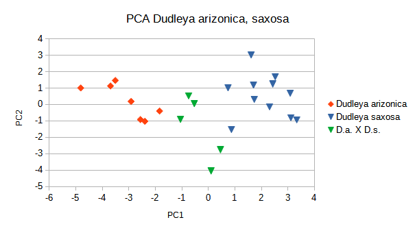
Fig. 1. Plot of the second principal component (PC2) vs. the first one (PC1).
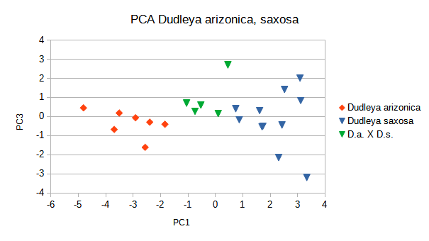
Fig. 2. Plot of the third principal component (PC3) vs. the first one (PC1).

Fig. 3. Plot of latitude vs. PC1 (the first component from the Principal Components Analysis).
Of course, the PCA doesn't label any of the points as a given taxon, so there is interpretation involved as to how to group the points. I've labeled the point as one of the species or as a hybrid based on all available evidence.
For example, one could certainly argue from the PCA alone that the hybrid specimen closest to the D. saxosa points (with PC1 = 0.46) might actually be part of the D. saxosa population. But the latitude of that specimen, as shown in Fig. 3, is well away from the D. saxosa population, and it is geographically close to another hybrid specimen with the smallest value of PC1. Both of those specimens are from Smuggler Canyon, nestled within the range of D. arizonica and outside the range of D. saxosa (see Figs. 2 and 3 on the results page). Finally, even within the PCA itself, both PC2 and PC3 indicate that there is something different about that PC1 = 0.46 specimen, with both having values outside of any in the D. saxosa population. Those arguments put together fairly strongly support labeling that specimen as a hybrid.
You can examine that specimen to see what you think, and the specimen of D. saxosa closest to it in PCA, in the compilation of all the photographs I measured.
I plan on adding more points to this analysis, which may, or may not, clarify the interpretation of the points. If the hybrids are not first generation (F1) hybrids and result from continued back-crossing with one of the parents, some specimens may be nearly impossible to distinguish from their parents.