Opuntia echinocarpa, O. ganderi, O. parryi, and O. wolfii: Analysis of How Well Non-Blooming Specimens Are Distinguished
Introduction
Data
Pictures of Specimens
Analysis
Principal Component Analysis
Analysis of Spines
Comparison to Descriptions in Floras
Conclusions
Introduction
For an introduction to these species, see Opuntia echinocarpa, O. ganderi, O. parryi, and O. wolfii: Locations and Pictorial Identification Guide.
* This analysis was done, and this page written, from my first day of fieldwork on these species. Since then, I have accumulated much more data on these species, but have retained this page essentially as it was written on 27 January 2007, except for a few comments and corrections noted below in italics prefaced by an asterisk, such as this paragraph you are reading. This page in its original form shows what can be learned in one day of fieldwork by someone who had never studied these species before and who was a complete novice at attempting to separate these species in the field. In particular, 9 of the 10 specimens were correctly determined in the field, and it turns out that the single incorrectly-determined specimen has fooled many other botanists as well from its superficial appearance!
On 23 January 2007 I measured ten specimens of these four species along Highway S2 to see how well easily-measurable characteristics of non-blooming plants could separate the species. In the field, I used the keys to non-blooming specimens given here to tentatively identify the specimens. The analysis presented here did not use any of the features in those keys, and thus provides independent objective evidence as to how well the species separate.
I was particularly interested in discovering whether any of the "O. parryi" or "O. ganderi" specimens would show evidence of the hybridization mentioned in the Flora of North America or in Rebman 2005. * See "Intergradation" between Opuntia parryi and O. ganderi for further information, and The transition between Opuntia parryi and O. ganderi along Highway S2 in San Diego County for a much more detailed later study to detect possible hybridization.
Specifically, I intentionally sampled three plants that were the most unusual specimens in the field at stops 2 and 3 in the area where hybrids had been reported, as well as sampling one average-looking specimen of O. parryi. At stop 4, I intentionally sampled the weakest-looking specimen as well as the most robust specimen of O. ganderi, judged primarily by stem diameter.
Data
For each specimen, I noted the number of main stems, and measured the minimum and maximum length and diameter of the stem segments for fully grown segments. I measured the length of the tubercles on the stem, and the width of the raised portion. Only one tubercle was measured on each specimen, since it is time-consuming to maneuver a ruler amidst the spines. I only realized during the later analysis that floras usually report the width of the entire tubercle, including the flat portion surrounding the raised portion, and hence readers should be aware that my measurements will be narrower than the width of the entire tubercle.
I noted the number of spines per areole on the stem, and the color of the spines, as well as how spiny the fruit were. I measured the length of the fruit, and its diameter at its maximum extent, which was always near the top. The fruit were all very dry. Only a single fruit was measured for each specimen, since many specimens had only a single fruit that could easily be measured.
The data are presented in the following two tables, along with the identification tentatively made in the field and notes on some specimens.
Cholla Measurements
| Spec- imen # | Stop # | GPS # | # Main Sts | St Segment Length (cm) | St Segment Diameter (cm) | Tubercle Length (mm) | Tubercle Rib Width (mm) | Fr Length (mm) | Fr Width (mm) | ||
|---|---|---|---|---|---|---|---|---|---|---|---|
| Min | Max | Min | Max | ||||||||
| 1 | 1 | 1 | 15 | 13 | 16 | 2.5 | 3 | 24 | 3 | 27 | 11 |
| 2 | 2 | 2 | 15 | 17 | 19 | 3 | 3.5 | 28 | 5 | 27 | 15 |
| 3 | 2 | 2 | 15 | 7.5 | 15 | 2 | 2.5 | 25 | 3 | 25 | 15 |
| 4 | 3 | 3 | 3 | 14 | 17 | 1.5 | 2 | 21 | 2 | 25 | 15 |
| 5 | 3 | 4 | 3 | 22 | 34 | 2.5 | 3 | 25 | 4 | 30 | 15 |
| 6 | 5 | 5 | 15 | 10 | 15 | 2 | 2 | 20 | 2 | 15 | 13 |
| 7 | 5 | 6 | 12 | 14 | 17 | 2.5 | 3 | 17 | 3 | 20 | 12 |
| 8 | 7 | 7 | 10 | 5 | 10 | 1.5 | 2.5 | 11 | 3 | 18 | 11 |
| 9 | 7 | 8 | 1 | 6.5 | 8 | 2 | 2.5 | 12 | 3 | 15 | 11 |
| 10 | 9 | 9 | 1 | 5 | 10 | 2 | 2 | 20 | 4 | 15 | 15 |
| 11 | 9 | 7 | 12 | 2 | 2 | ||||||
| 12 | 9 | 5 | 10 | 2.5 | 2.5 | ||||||
| 13 | 9 | 5 | 9 | 1.7 | 2.1 | ||||||
| 14 | 9 | 7 | 10 | 2 | 2.5 | ||||||
| 15 | 9 | 8 | 10.5 | 1.7 | 2.5 | ||||||
Cholla Specimen Spine Characteristics And Additional Comments
| Spec- imen # | Field Determination | Comments |
|---|---|---|
| 1 | O. parryi | A typical specimen in this area. Spines tan, subequal, not robust, ~half tubercle length |
| 2 | O. parryi | A spinier-than-normal specimen in this area. Spine along tubercle center more robust than others, but only slightly longer |
| 3 | O. parryi | A much-spinier-than-normal specimen in this area. Spines tan except for one along tubercle center which is much more robust and much longer than others, longer than tubercle |
| 4 | O. parryi | Specimen much taller than others, ~6 feet (2 m); spines subequal, tan, about as long as tubercle, but with some whitish slightly longer spines along tubercle; fr moderately spiny |
| 5 | "O. ganderi"* | Spines unequal, tan, longest equal to tubercle length, not entirely obscuring tubercles |
| 6 | O. ganderi | Specimen selected as one with the narrowest stem segments in this area that also contained specimen #7. Spines unequal, one along tubercle center much more robust and much longer than others, longer than tubercle |
| 7 | O. ganderi | Specimen selected as one with the widest stem segments in this area that also contained specimen #6. Spines white to tan, unequal, one along tubercle center much more robust and much longer than other, longer than tubercle |
| 8 | O. wolfii | Spines very unequal, longest much longer than tubercles and much more robust than other spines |
| 9 | O. wolfii | Spines very unequal, white to tan, longer spine much longer than tubercles |
| 10 | O. echinocarpa | Spines very unequal, white to gold, two much longer than tubercles and more robust |
* This specimen is actually O. parryi, but I mistakenly thought it was O. ganderi in the field and in the plots given below in the original analysis.
Only specimens 1-10 were completely measured. Specimens 11-15 were just measured for their stem segments and tubercles, to get an estimate of the range for those characteristics for O. echinocarpa.
All fruit were densely spiny except for #3 which had moderately spiny fruit. All spines were white except as noted. The number of spines per areole was always ~10-20.
The GPS locations for each specimen are given in the following table, and plotted in the following map. Note that locations 1 and 2, 3 and 4, 5 and 6, and 7 and 8 are very near to each other, and hence plot on top of each other in the map.
GPS Locations (decimal degrees, NAD27)
| GPS # | Latitude (deg; N) | Longitude (deg; E) | Elevation (feet) |
|---|---|---|---|
| 1 | 33.15732 | -116.54993 | 2760 |
| 2 | 33.15534 | -116.54740 | 2720 |
| 3 | 33.09663 | -116.47342 | 2280 |
| 4 | 33.09649 | -116.47352 | 2280 |
| 5 | 33.03467 | -116.41097 | 2580 |
| 6 | 33.03465 | -116.41091 | 2580 |
| 7 | 32.82827 | -116.16671 | 1230 |
| 8 | 32.82817 | -116.16677 | 1230 |
| 9 | 32.78896 | -116.10160 | 910 |
Map Showing GPS Locations

Pictures of Specimens
Entire Plant
| #1 | 
|
| #2 | 
|
| #3 |  #3 is the spinier plant on the right; compare to normal O. parryi specimen at upper left which is growing immediately next to #3 |
| #4 | 
|
| #5 | 
|
| #6 |  #6 is the plant on the left |
| #7 | 
|
| #8 | 
|
| #9 | 
|
| #10 | 
|
Stem and Fruit
| #1 |  | 
|
| #2 | 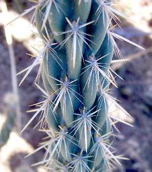 | 
|
| #3 |  | 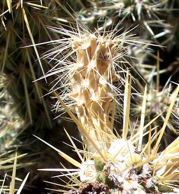
|
| #4 |  | 
|
| #5 |  | 
|
| #6 | 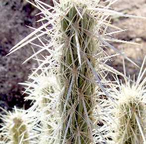 | 
|
| #7 |  | None photographed |
| #8 |  | None present |
| #9 | 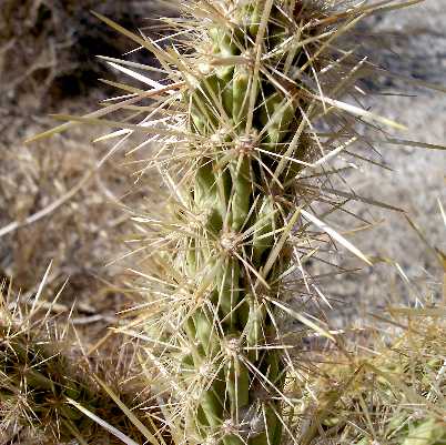 | 
|
| #10 |  | 
|
Analysis
Principal Component Analysis
Eight characteristics measured for each of the ten specimens were analyzed using Principal Component Analysis (PCA): the minimum and maximum stem segment length and width, the tubercle length and width, and the fruit length and width. For specimen #10, for its stem segment width, I substituted the range of 1.7 to 2.5 cm measured for nearby specimens for the single value of 2.0 cm measured on that specimen, a minor change.
PCA is a just a simple way to look at the total variation in the data set to see how well the data samples separate. Humans can easily look at the total variation when there are only two characteristics measured, but it becomes increasingly difficult for us to analyze data sets with larger numbers of measured characteristics.
With two characteristics, PCA corresponds to simply fitting a line to the data where one characteristic is plotted against the other. PCA then rotates the plot so that the line corresponds to the new x-axis. It does this by making new variables that are linear combinations of the two characteristics. The values for Principal Component 1 (PCA 1) are then just the new x values, and the values for Principal Component 2 (PCA 2) are then just the new y values. I.e., to obtain PCA 1, PCA finds the correlation among variables that produces the maximum variance (spread) in the data, and defines a new variable, PCA 1, that is a linear combination of the variables aligned with the direction of maximum variance.
In higher dimensions, PCA does the same thing for PCA 1, but then continues the search for maximum variance after removing the variance captured by PCA 1. With most data sets, nearly all the variance is captured by the first 2-3 components.
I.e., PCA is just a fancy term for capturing the correlation of multidimensional data into a small number of variables that the human mind can better deal with.
In this analysis, PCA 1 captured 80% of the total variance in the entire data set; PCA 2 captured 12%; and PCA 3 captured 5%. Between them they accounted for 97% of the total variance.
The following plots show how the ten specimens separate using the first three principal components. The points are colored according to the field determinations, and individual specimens of O. parryi and O. ganderi are labeled.
If the stem, tubercle and fruit characteristics have different relationships between the species, they should fall into groupings in these plots. If so, and if the field determinations are correct, colored points should form separate groupings. If the field determinations are incorrect, the colored points will not form groups; some will be mixed with points of other colors.
Any hybrids that are present should plot intermediate to the parent species.


As can be seen, the points cluster according to the determinations made in the field except that specimen #5 stands apart from all other species in PCA 1.
* In my original analysis, I used the plot of PCA 3 vs. PCA 2 to "confirm" the identify of #5 as "O. ganderi", but that turned out to be incorrect. Further analysis of many more measured specimens showed that #5 turned out to be connected to the other O. parryi points in the plot of PCA 2 vs. PCA 1, and was distinct from the other O. ganderi points. A difference in PCA 1 is much more significant than a difference in PCA 2 and PCA 3.
Thus the objective measurements of dimensions of the stems, tubercles and fruit confirm those species assignments * except for specimen #5. Each of the four species has its own area delineated in the plots.
Furthermore, there is no evidence that the unusual-looking O. parryi specimens have any hybridization with O. ganderi. In the PCA 3 vs. PCA 2 plot, the O. parryi and O. ganderi groups of points have greater separation from each other than from the points of any other species. In particular, specimen #3 of O. parryi, thought in the field to look like it might have some hybridization with O. ganderi, is the farthest from the O. ganderi region in the plots.
Only in the variable PCA 1 do the specimens of O. parryi and O. ganderi overlap, which is why they are thought to be similar to human eye in the field. PCA 1 is simply a size parameter, which is one of the things to which the human eye is quite sensitive.
O. parryi and O. ganderi both have longer stem segments, thicker stems, longer tubercles, and longer fruit, and hence both species have large values for PCA 1. Specimen #5, of O. ganderi had the longest stem segments by far, which accounts for its having the largest value of PCA 1 by far (* such a long stem segment length is in fact only consistent with O. parryi, as I later found out by measuring many other specimens of both species!)
I did not use the height of the plants in the PCA, since that is often environmentally induced as well as age related. For example, specimen #4, taller by a factor of two than the other specimens, looks quite average for its value of PCA 1. It simply grew larger while retaining the fundamental characteristics of its species.
The variables PCA 2 and PCA 3 pick up more subtle distinctions in the species, not immediately apparent to the human eye. The values of the coefficients for these three variables are given in the next table.
Coefficients of the Principal Component Variables 1 To 3
| Characteristic | PCA 1 | PCA 2 | PCA 3 |
|---|---|---|---|
| St segment length min (cm) | 0.47 | 0.31 | 0.01 |
| St segment length max (cm) | 0.62 | 0.48 | 0.31 |
| St segment width min (cm) | 0.03 | -0.01 | 0.00 |
| St segment width max (cm) | 0.02 | -0.01 | -0.04 |
| Tubercle length (mm) | 0.41 | -0.76 | 0.39 |
| Tubercle width (mm) | 0.03 | -0.04 | 0.03 |
| Fr length (mm) | 0.47 | -0.26 | -0.81 |
| Fr width (mm) | 0.09 | -0.18 | 0.33 |
PCA 1 sums up the correlated variation of the above variables. Since all coefficients for PCA 1 are positive, this implies that all these quantities grow larger together among all the species, as would be expected. (The value for PCA 1 for each specimen is arrived at by multiplying the coefficient from the table above times the corresponding measurement for that specimen, summing over all characteristics and then subtracting the mean for all specimens.)
PCA 2 is essentially the stem segment length (note the large positive values of the coefficients for the minimum and maximum stem segment length) minus {the tubercle length plus the fruit length and width}. Thus it picks up the species-specific variations in the relationships of those characteristics, such as one species having characteristically shorter fruit and longer stem segments. PCA 3 picks up a different species-specific variation by essentially taking the stem segment length plus the tubercle length minus the fruit length.
The human brain does not easily pick up such distinctions in the field, nor is it easy to make a simple plot of one characteristic against another to see this separation.
It is easy to see how different O. wolfii and O. echinocarpa are from the other two species. The stem segments for those two species were all 10 cm or less in length, whereas the other two species had at least one stem segment 15 cm or greater. Also, O. wolfii had the shortest tubercle lengths by far, 11-12 mm, with the other species having tubercles 17 mm or longer. These differences were so striking that it was immediately apparent in the field as I made the measurements.
Unfortunately, there is no easy way to show the discrimination picked up by PCA 2 and PCA 3 between O. parryi and O. ganderi.
Interestingly, the distinction used in the Jepson Manual to separate O. parryi, St gen < 2 cm diam, proved unreliable in distinguishing this species. I measured stem segments of 1.5-3.5 cm, with only a single specimen having stem segments narrower than 2.0 cm. The other three species had stem segments of 1.5-3.0 cm, essentially the same values.
I did not include the spininess of the fruit in this analysis, since the field measurements showed all fruits had essentially the same spininess for all species. The Flora of North America separates O. parryi on Spines 0-few per fruit, yet the fruits are all quite spiny, with ~100 or more spines per fruit.
Analysis of Spines
The characteristics of the spines did not enter either in the field determination or in the analysis above. Most of the spine characteristics listed in the table above were derived from later analysis of the photographs shown above. Hence they are an independent check on how separate these plants are.
The appearance of the spines alone group the specimens into three categories which follow the species delineations in the field except for not distinguishing O. wolfii and O. echinocarpa (* and failing to distinguish specimen #5 as O. parryi. However, with a much more experienced eye now, I can see a distinct difference in the spininess of the entire plant in the pictures above.)
Spines of specimens of O. parryi form a series of "short equal spines" to "moderate-length equal spines", as well as a series of "short equal spines plus one largish spine" to "moderate-length equal spines plus one largish spine". Most of the spines of O. parryi are much less robust than the typical spines of the other species.
Spines of specimens of O. ganderi all have large unequal spines, recognizably different from any specimen of O. parryi. Spines of specimens of O. wolfii and O. echinocarpa have some very long spines, different from both O. parryi and O. ganderi.
Comparison to Descriptions in Floras
In the following, I have converted the English system measurements in Benson (1969) to metric equivalents.
O. echinocarpa. My single measured tubercle length was 20 mm, larger than 4-13 mm in the Flora of North America and the 6-10 mm in Benson.
A minor comment: measured stem segments lengths are 5-10 cm. The maximum length of 10 cm is larger than the typical maximum stem segments of 7.5 cm for the terminal stem segments given in the Flora of North America and the 8 cm given in Benson. But my measurements are within the infrequent largest segment of 12 cm given in the Flora of North America and 15 cm given in Benson.
O. ganderi.
- Measured stem segment lengths are 10-19 cm (* this has been corrected from 10-34 cm by removing #5). Interestingly, there is almost no overlap between the 20-50 cm in Benson and the 10-26 cm in the Flora of North America.
- Measured stem segments widths are 2.0-3.0 cm, slightly smaller than the 2.5-4.5 cm in the FNA, and not overlapping with the 3-4 cm in Benson.
O. parryi.
- Measured stem segments widths are 1.5-3.5 cm, larger than the 1.5-1.9(2.5) cm in Benson, or the 1.5-2.5 cm in the Jepson Manual and the Flora of North America.
- The fruit is moderately to densely spiny, with ~100 spines or more, not the Spines 0-few per fruit given in the Flora of North America key. (The Jepson Manual says the fruit is variably spiny.)
A minor comment: the dried fruit is 11-15 mm wide, not the 13-26 mm of the Flora of North America.
O. wolfii.
- Measured stem segment lengths are 5-10 cm, slightly smaller than the 6-40 cm in the Flora of North America, but much smaller than the 10-25 cm in Benson.
- Measured tubercle lengths are 11-12 mm, within the 10-15 mm of the Flora of North America, but much smaller than the 15-25 mm in the Jepson Manual, which doesn't overlap with the Flora of North America range.
Conclusions
The above analysis shows that field determinations using a simple key to non-blooming specimens are apparently reliable in determining the species of a given specimen (* except for a single specimen of O. parryi). The field determinations were strongly confirmed by Principal Component Analysis using independent objective measurements of the length and width of stem segment length, tubercles, and fruit. The determinations were further confirmed for three of these four species by analysis of the spines; only O. wolfii and O. echinocarpa could not be immediately separated by their spines.
Furthermore, for O. parryi and O. ganderi, this study was done using a challenging data set. In two locations in an area where possibly hybrids between those species had been reported, I intentionally selected specimens that looked most different from the typical specimen for each species in those areas. In a third location I also selected the two extreme specimens of O. ganderi. Yet no difficulties were found in determining the species for each of the challenging specimens.
Hybrids between O. parryi and O. ganderi may of course exist, but this analysis shows that they are not picked out by selecting non-flowering specimens on the basis of their difference from neighboring plants. In particular, the striking specimens of O. parryi that are spinier than typical plants, or much taller than typical plants, are clearly part of the normal variation within the O. parryi population.
It is of course still possible that variations seen in the flowers might reveal evidence of hybridization. It is also possible that the variance within these two species themselves has not been fully recognized.
Surprisingly, the two main distinctions used to separate O. parryi in the Jepson Manual and the Flora of North America totally fail for the population studied here. The Flora of North America separates O. parryi on Spines 0-few per fruit, yet the fruits are all quite spiny, with ~100 or more spines per fruit. The Jepson Manual separates O. parryi on St gen < 2 cm diam, yet my specimens gen had stems wider than 2.0 cm diam up to 3.5 cm.
I intend to analyze other populations of O. parryi in the near future to see how closely they resemble this population. Coastal specimens have previously been defined as O. bernardina; perhaps those specimens more closely resemble the descriptions in the floras for "O. parryi".
I thank Wayne Armstrong, Dave Stith, Norrie Robbins, and Kate Shapiro for help with the fieldwork on 23 January 2007, as well as for kindly providing good scale information in some of the above pictures, even though the upper parts of the bodies didn't always survive the cropping.